Using the IR light source and IR filters we now have a clear separation of signal and noise from our camera. Now we can get to the task of detecting marker positions.

First we'll convert the luminance image into a thresholded binary image. Finally, this image is converted into a list of marker positions.

Experiment

Before codifying marker recognition, let's first experiment a bit. We'll be detecting spherical markers:

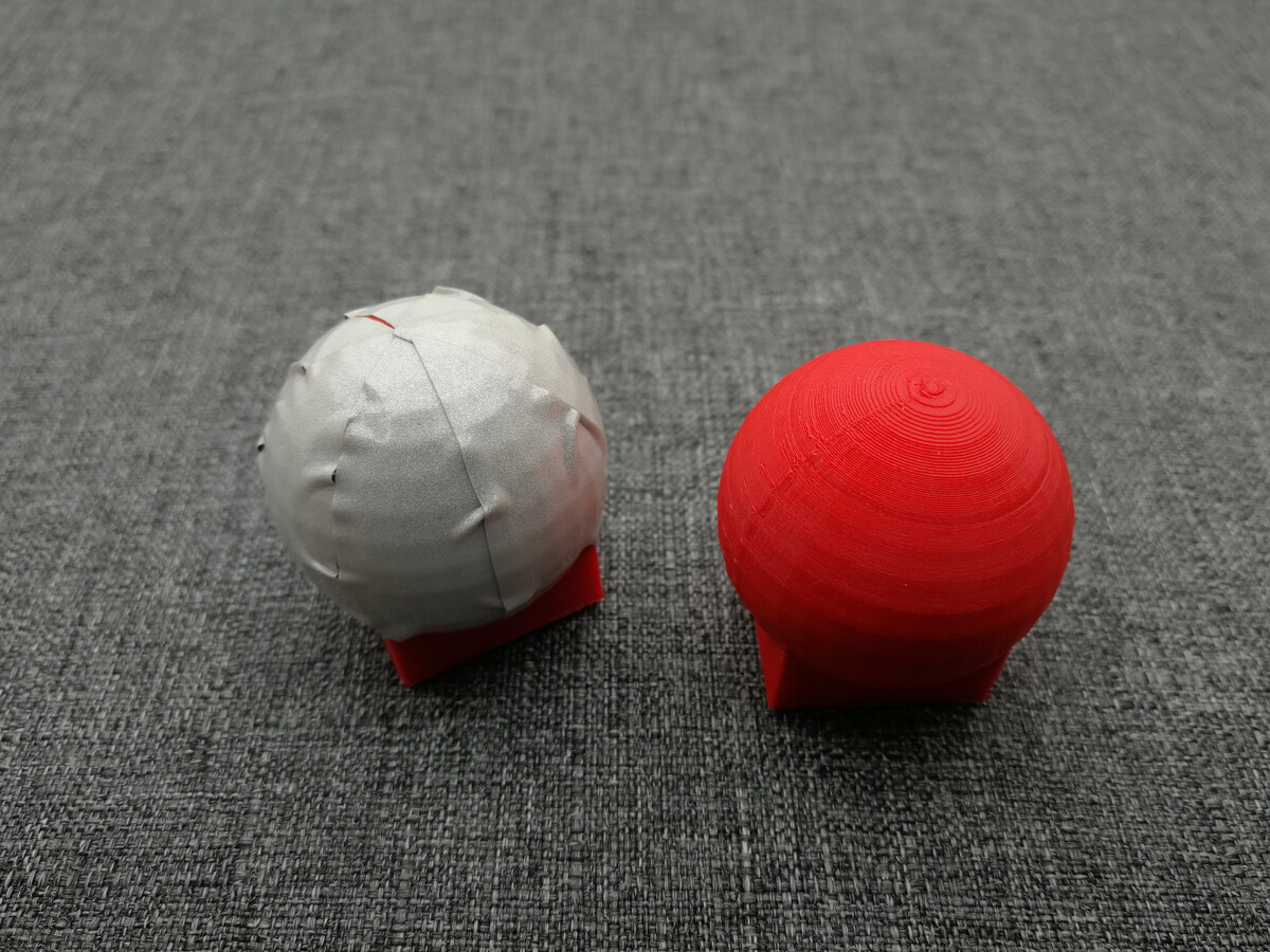
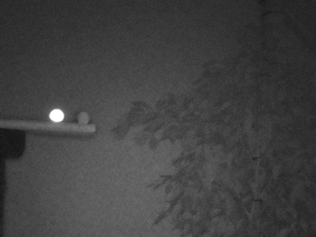
One marker has been coated in reflective tape the other is simply the mildly reflective PLA print material. In a future post we'll look at the 3D model, cut out templates and different reflective materials. For now, let's look how a single frame from the camera looks:

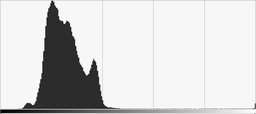
From the frequency diagram it is pretty clear that distinguishing the marker pixels from the image is exceptionally simple. A simple threshold value any where between 128 and 250 will filter only the marker:

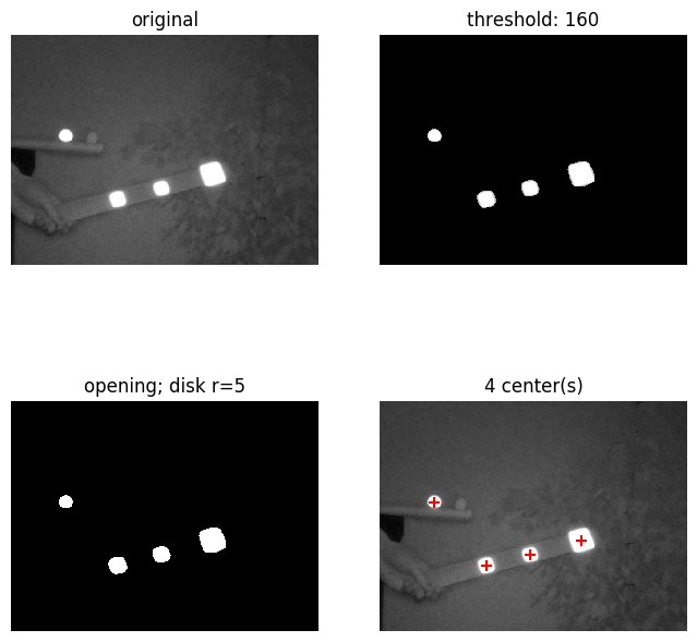
As you can see, with a threshold of 160 we get a perfect binary image. Having such a perfect result with such a range of thresholds is superb. I promise you that image recognition is normally a lot harder than this! It shows the importance of using a IR light source and IR pass filter.

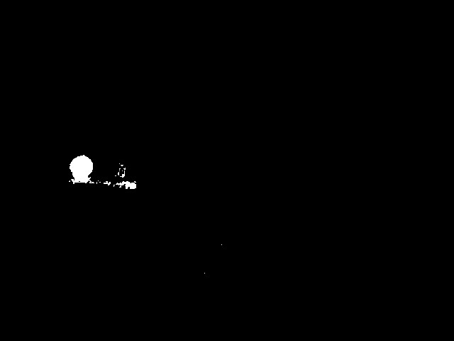
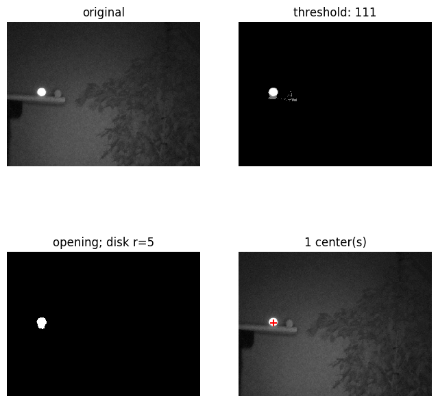
To increase robustness of further steps I'm going to murky the results of this step a bit. Say somehow a bit more noise came true, such as with a threshold of 111, how do we deal with this and how can we extract the marker center?

Noise reduction

To get rid of the noise we can do a morphological opening. This will open up parts of the image that are small and of a different shape than our template.

Scikit-image morphology can do this operation for us.

It is quite a long operation though. On my fast laptop the operation with a disk of size 5 takes almost 30 of the total 40ms processing time:

Threshold	0.1ms
Opening	27.0ms
Connect	1.1ms
Center	13.6ms
Total	41.9ms

We might be able to speed this step up at a later time, for now let's use this and move on to extracting the position.

Position extraction

The final step to get the marker position entails calculating the center of all remaining pixel blobs. This is a two step process:

1. Find all connected components, that is: all pixel blobs.
2. Compute center of these connected components.

Again we can use a library to do the heavy lifting for us.

• The scipy.ndimage.label function performs a connected component analysis.
• Next the scipy.ndimage.center_of_mass function calculated the center of mass, multiple objects at the same time.

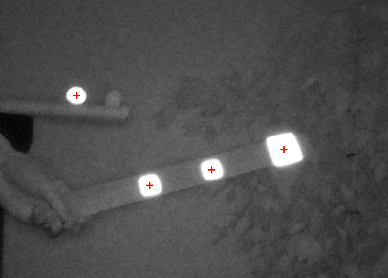
The result is the extracted marker position:

Code

All described steps are performed with the following experimental code:

"""
Detect markers in image and display results
"""
import time
import numpy as np

import matplotlib.pyplot as plt
from scipy import ndimage
from skimage import io
from skimage import morphology


def do_threshold(array, value):
    return (array >= value) * array


def difference_ms(prev_t):
    return round((time.time() - prev_t) * 1000, 1)


def main(path):
    original = io.imread(path)

    threshold = 160
    opening_size = 5

    t0 = time.time()
    thresholded = do_threshold(original, threshold)  # very slow
    print(f'Threshold:\t{difference_ms(t0)}ms')

    t1 = time.time()
    structure = morphology.disk(opening_size)
    opened = ndimage.binary_opening(thresholded, structure)  # quite slow
    structure = np.ones((3, 3), dtype=np.int)
    print(f'Opening:\t\t{difference_ms(t1)}ms')

    t2 = time.time()
    labels, ncomponents = ndimage.label(opened)  # fast
    print(f'Connect:\t\t{difference_ms(t2)}ms')

    t3 = time.time()
    centers = ndimage.measurements.center_of_mass(opened, labels, range(1, ncomponents + 1))  # fast
    # Note, performing moment calculation on masked image may be faster (parallelizable).
    print(f'Center:\t\t\t{difference_ms(t3)}ms')

    total_ms = difference_ms(t0)
    print(f'Total:\t\t\t{total_ms}ms')

    print(f'ncomponents: {ncomponents}')
    print(f'centers: {centers}')

    #
    # Plot
    #
    fig, axes = plt.subplots(2, 2, figsize=(8, 8), sharex=True, sharey=True)

    axis = axes[0, 0]
    axis.imshow(original, cmap=plt.cm.gray)
    axis.set_title('original')
    axis.axis('off')

    axis = axes[0, 1]
    axis.imshow(thresholded, cmap=plt.cm.gray)
    axis.set_title(f'threshold: {threshold}')
    axis.axis('off')

    axis = axes[1, 0]
    axis.imshow(opened, cmap=plt.cm.gray)
    axis.set_title(f'opening; disk r={opening_size}')
    axis.axis('off')

    axis = axes[1, 1]
    axis.imshow(original, cmap=plt.cm.gray)
    axis.set_title(f'{ncomponents} center(s)')
    axis.scatter(np.array(centers)[:, 1], np.array(centers)[:, 0], s=50, c='red', marker='+')
    axis.axis('off')

    # fig.suptitle(f'Total {total_ms}ms', fontsize=12)
    # fig.tight_layout(rect=[0, 0.03, 1, 0.95])

    plt.savefig('plot.png', bbox_inches='tight')
    plt.show()

    fig, axis = plt.subplots(1, 1, figsize=(8, 8), sharex=True, sharey=True)
    axis.imshow(original, cmap=plt.cm.gray)
    axis.scatter(np.array(centers)[:, 1], np.array(centers)[:, 0], s=50, c='red', marker='+')
    axis.axis('off')
    plt.savefig('result.png', bbox_inches='tight')


if __name__ == "__main__":
    path = 'luminance_raw_with_IR_light.jpg'
    path = 'more-marker-raw_IR_light.jpg'
    main(path)

Link to gist

The same pipeline performed on multiple markers:

Concluding

By thresholding, opening and computing the centroid of the connected components we can effectively get the marker positions. There are still some drawbacks right now, mostly the time spend on the opening and centroid calculation is quite high.

But less push on for now, the next challenge is to detect markers with the real time recording on the Raspberry Pi itself.